
Introduction to Computational Complexity Theory
Understanding the Limits of Computation, One Step at a Time


In the whole history of computer science, very few ideas have reshaped our thinking as profoundly as the concept of complexity.
We’re not talking about complexity in the colloquial sense, like the messy, confusing, or chaotic, but a precise mathematical framework to ask one of the most fundamental questions in all of computing:
How hard is it to solve a problem?
This is the beating heart of computational complexity theory. At first glance, the question might sound a bit trivial. Give me a program and an input, and I’ll run it, so what’s the problem?
But take your time, dig a little deeper, and you’ll find a whole universe of nuance. Some problems that seem simple in theory are, in fact, completely intractable.
Others that appear insurmountable can be solved in a few milliseconds. Complexity theory, which is a subset of computability theory, is the field that formalizes this intuition and provides the tools to map the boundaries of what’s efficiently computable in an effective and finite period of time.
To do that, we need a new kind of microscope; not one that examines what a program does, but how much it costs to do it.
In traditional programming, we’re often concerned with correctness. Does the program produce the right output for a given input? If yes, great! All you need to do is to ship it.
But in complexity theory, correctness is only the starting line. We need to zoom out and ask ourselves:
how many steps does the program take?
How much memory does it consume?
What happens as the input grows larger and larger?
These questions don’t just shape how we write programs, they rather define whether a problem is even feasible to solve at all.
This is the shift: from functionality to scalability, from does it work? to does it scale?
Imagine a program that solves a problem perfectly, only, it takes a billion years to run for inputs larger than a few dozen elements.
Technically it’s correct, but practically useless. That’s where complexity theory steps in: it gives us the practical (and even technical) tools to measure and categorize this kind of “computational cost.”
Think of it like this: if computer science is the study of what can be computed, then complexity theory is the study of how efficiently it can be done.
So let’s begin. Let's put our algorithmic systems under this microscope and take our first look at the anatomy of complexity.
The Cost of Computation
Let’s start with a simple toy example.
Suppose I give you a list of numbers and ask you to find the largest one. Sounds pretty easy, right?
def max_element(lst):
    max_val = lst[0]
    for x in lst:
        if x > max_val:
            max_val = x
    return max_val
This program is clear and effective. But we’re not here to admire its astonishing elegance, we’re here to analyze it. How long does it take to run?
If you give it a list of length 10, it checks 10 numbers. If you give it a list of 1,000, it obviously has to check 1,000 times. There’s a linear relationship between input size and time. We say the algorithm has linear time complexity, simply denoted as O(n).
In complexity theory, we abstract away the details of specific machines and implementations. Instead, we ask:
how does the number of basic steps grow as a function of the input size?
That’s the core idea. It’s pretty simple, but it’s actually incredibly powerful.
Defining Complexity Classes
Now that we can talk about the “cost” of algorithms, we can start categorizing problems based on how expensive they are to solve.
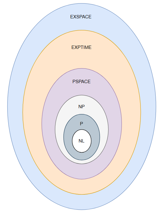
Let’s now take some time to define some fundamental complexity classes. Think of these as boxes that contain problems with similar difficulty profiles.
Here we have:
NL (Nondeterministic Logarithmic Space)
Decision problems solvable by a nondeterministic Turing machine using logarithmic space. Formally, a language L∈NL if there exists a nondeterministic Turing machine that decides L using O(log n) space.
Example: s-t reachability in a directed graph (can you reach node t from node s?).
Key fact: NL ⊆ P, and due to the Immerman–Szelepcsényi theorem, NL = co-NL.
NL captures problems that are highly space-efficient but potentially time-consuming in practice.
P (Polynomial Time)
Problems solvable in polynomial time on a deterministic Turing machine.
Formally, L∈P if there exists a deterministic machine that decides L in time O(n^k) for some constant k.
These are “efficiently solvable” problems in classical complexity theory.
Notable examples include: Sorting, searching, matrix multiplication, shortest path (Dijkstra's algorithm).
NP (Nondeterministic Polynomial Time)
Problems for which a solution can be verified in polynomial time by a deterministic machine, or equivalently, solved in polynomial time by a nondeterministic Turing machine.
L∈NP takes shape if there exists a polynomial-time verifier V(x,y), where x is the input and y is a certificate or witness.
Includes decision problems like SAT, clique, and Hamiltonian cycle.
Open problem: Does P = NP?
PSPACE (Polynomial Space)
Problems solvable with a polynomial amount of memory, regardless of time.
Formally, L∈PSPACE if a deterministic Turing machine decides L using space O(n^k).
PSPACE includes all of P and NP, but also more complex problems such as QBF (Quantified Boolean Formula).
Example: Determining if a player has a winning strategy in generalized chess.
EXPTIME (Exponential Time)
Problems solvable by a deterministic Turing machine in time 2^[p^(n)] for some polynomial p(n).
In formal ways, L∈EXPTIME if there is a TM that decides L in time O(2^[n^k]).
Contains problems like generalized games (e.g. chess on an n×nn \times n board) and exact algorithms for logic-based models.
Strictly contains P, and under standard assumptions, P ⊂ EXPTIME.
EXPSPACE (Exponential Space)
Problems solvable using exponential memory, i.e., space 2^[p^(n)].
We can say that L∈EXPSPACE if it can be decided by a Turing machine using O(2^[n^k]) space.
Includes logic-heavy problems and high-order model checking tasks.
Like EXPTIME, this class is believed to be strictly larger than PSPACE:
PSPACE ⊂ EXPSPACE, and EXPTIME ⊂ EXPSPACE.
So What Does It All Mean?
Among all the elegant boxes of complexity classes we can draw (NL, P, NP, PSPACE, EXPTIME, EXPSPACE) P vs NP is the GOAT: the greatest of all theoretical challenges, a question that feels less like a technical footnote and more like a philosophical puzzle about the nature of reasoning itself.
NP-completeness is much like a kind of computational badge of honor, a signal that a problem sits on the bleeding edge of what’s efficiently solvable.
It’s not just hard; it’s universally hard. If you solve one NP-complete problem efficiently, the dominoes fall: suddenly, every problem in NP gets an efficient solution, too.
This isn’t just an academic exercise. These problems lurk everywhere, in logistics, cryptography, artificial intelligence, circuit design, game theory. If your program is running slow and you’re not sure why, you may have stumbled into NP-complete territory.
And yet, life goes on. Despite the seemingly grim computational outlook, we solve these problems all the time. Just... not perfectly.
Engineers wield heuristics, approximations, and problem-specific tricks like carpenters with tool belts. If we can’t solve it fast, we’ll settle for close enough, and most of the time, that’s good enough.
Beyond the Cliff’s Edge: NP-Intermediate and NP-Hard
Not all hard problems are NP-complete. Some, like the Graph Isomorphism problem or integer factorization, sit in a murky middle ground: not known to be in P, not known to be NP-complete.
These are called NP-intermediate problems, they only exist if P ≠ NP, but assuming they do, they’re the rebels that resist classification.
And then there’s NP-hard, a kind of superset. These problems are at least as hard as the hardest problems in NP, but they may not be in NP themselves. For instance, chess, checkers, or Go, when framed as decision problems over arbitrary-sized boards, are NP-hard but not in NP.
Why? Because verifying a solution isn’t always easy (or even possible in finite time).
So, here’s a short take:
NP: "I can verify it quickly if you show me the answer."
NP-complete: "I’m the hardest among the quickly-verifiable."
NP-hard: "I’m at least as hard as that, and maybe harder."
P: "I can both find and verify the answer quickly."
Why We Obsess Over P vs NP
The P vs NP question isn’t just a theoretical brainteaser. It’s the moonshot of computer science. If P = NP, it means we could suddenly find computationally efficient solutions to thousands of problems we currently consider intractable.
But it would also break the foundations of modern cryptography. Passwords, digital signatures, encrypted messages, all of them depend on the assumption that some problems are just too hard to solve quickly.
On the other hand, if P ≠ NP, then there are limits. Concrete, provable boundaries to what can be solved efficiently.
It’s a sobering thought, but also clarifying. It tells us which battles to pick, which shortcuts to take, and when to stop chasing a perfect answer.
Either way, solving the P vs NP problem is worth a million dollars, and a permanent spot in the annals of mathematics and computer science.
A Glimpse at NP-Completeness
Time for a twist in the plot.
Imagine for a while that you found a clever trick to solve just one problem in NP, not verify a solution, but actually compute one, in real polynomial time.
So…. You may be wondering to yourself, “Now, what happens?”
Let’s take some more time to find out.
You don’t just win infinite fame and an entire fortune (though yes, that $1,000,000 Clay Millennium Prize would be yours).
You trigger a seismic shift in computer science. You collapse a boundary that has stood for decades: the insurmountable boundary between P and NP.
Why? Because of a beautiful, terrifying idea known as NP-completeness.
Solve P vs NP, and you won’t just be celebrated; you’ll be truly immortalized. You’ll be remembered as one of the greatest mathematicians (or computer scientists, if you prefer) who ever lived. Your name will echo through history books, embedded in curricula, engraved in granite.
Entire generations of researchers will compare you to Alan Turing, calling you the Turing of the 21st century, not merely for what you solved, but for how you reshaped the very notion of what can be solved.
And after that? Sure, the Clay Institute will hand you a $1,000,000 check. But maybe, just maybe, you’ll take a different path. Maybe you’ll pull a Grigori Perel’man.
The man who solved the Poincaré Conjecture, and then turned his back on all the accolades, once said:
“I’m not interested in money or fame; I don’t want to be on display like an animal in a zoo.”
And more chillingly:
“Emptiness is everywhere and it can be calculated, which gives us a great opportunity. I know how to control the universe. So tell me, why should I run for a million?”
Solve P vs NP, and the universe itself might seem a little more calculable. But whether you accept the million or walk away from it like Perel’man, you’ll still be a legend.
(Sorry, we’re getting a bit carried away. Let’s get back to the main point…)
You basically collapse a boundary that has stood for decades: the boundary between P and NP.
Why? Because of a beautiful, terrifying idea known as NP-completeness.
NP-Complete: The Pinnacle of Difficulty in NP
NP-complete problems are not just “ a bunch of hard problems in NP”, they are the hardest. If you can crack one of them quickly (i.e., in polynomial time), you can crack every problem in NP just as efficiently. That’s the punchline.
But how did we get here?
Let’s rewind to the 1970s. In 1971, Stephen Cook, followed soon by Leonid Levin and Richard Karp, formalized this idea. They showed that the Boolean satisfiability problem (SAT) is NP-complete.
SAT asks: Given a logical formula (like
A ∨ ¬B ∧ C), can you assign true/false values to the variables so that the formula evaluates to true?
SAT doesn’t sound threatening. But it sits at the center of computational hardness. Once SAT was proven NP-complete, a torrent of other problems followed. Karp listed 21 in his famous paper, including:
Traveling Salesman
Knapsack
Graph Coloring
Subset Sum
Job Scheduling
Each of these is a wolf in sheep’s clothing. They look simple, even friendly. But if you try to solve them exactly for large inputs, you’ll run headfirst into computational chaos.
The Turing Machine: Why This Matters
To define the major complexity classes, we need a foundation that’s stripped of technological noise. No RAM, no GPUs, no compiler optimizations, no multithreaded runtimes humming beneath the surface. Just the bare minimum necessary to compute anything that’s computable.
Say hi to the Turing Machine.
Devised by Alan Turing in 1936, it’s an abstract, idealized model of computation. At first glance, it looks almost childishly simple:
An infinite tape divided into cells, each holding a symbol
A read/write head that moves left or right, one cell at a time
A finite set of internal states, and a table of transition rules governing what to do based on the current state and symbol
And… yeah that’s it.
No registers. No operating system. Just a machine that reads and writes symbols, moves its head, and switches states.
But that simplicity is its strength.
“What we want is a machine that can carry out any computation which can be described in symbolic terms.”
— John von Neumann, 1945, in a draft proposal for the EDVAC computer
Von Neumann, one of the founding architects of digital computing, understood the need for a universal model, something agnostic to implementation details. Turing’s invention provided exactly that.
Despite its minimalism, the Turing Machine is universal. That is, it is able to simulate any algorithm that can be executed on a modern digital computer. Anything you can code in Python, write in assembly, or compile to silicon can, in theory, be implemented on a Turing Machine, albeit very, very slowly.
“It is possible to invent a single machine which can be used to compute any computable sequence.”
— Alan Turing, 1936
This insight became the backbone of theoretical computer science.
And here’s the real kicker: if you can’t solve a problem on a Turing Machine with reasonable resources, say, in polynomial time or logarithmic space, then no amount of clever engineering will help.
Not even hyperscale data centers or quantum processors (unless, of course, we start redefining our entire model of computation).
By reducing everything to the Turing Machine, we give ourselves a ruler that is fair, rigorous, and untainted by hardware fads. It's the cleanroom of complexity theory.
If an algorithm fits into P on a Turing Machine, it’s fast by definition, not just because your laptop is powerful. If a problem demands exponential time or space, probably it’s not an artifact of bad coding; that’s the nature of the problem itself.
This is why all the major complexity classes (P, NP, PSPACE, EXPTIME…..), and the rest, are defined in terms of what a Turing Machine can or cannot do within certain limits.
We’re not interested in accidental slowness due to cache misses or bad compilers/IRs. We’re interested in fundamental limits, like what computation is and what it costs, at its most elemental level.
And so, in a world that changes hardware every few years, the Turing Machine endures, not because it’s realistic, but because it’s eternal.
Reductions: Building the Map of Hardness
When you first step into computational complexity, it feels like there’s a zoo of problems (SAT, 3-SAT, Clique, Vertex Cover, Hamiltonian Path…..) all different, all difficult, all frustratingly nuanced.
But then someone hands you a secret decoder ring: reduction.
Reductions are how complexity theorists talk to each other. They’re not just technical tools; they’re a language for expressing relationships between problems.
With a good reduction, you don’t need to solve a new problem from scratch. Instead, you transform it into something you already understand.
At its core, a reduction is like a translation. If you can take any instance of problem A and turn it into an instance of problem B efficiently, such that solving B gives you a solution to A, then we say A reduces to B.
And that one sentence is the beating heart of how we classify modern computational hardness.
This is where things get really elegant.
Say you have a hard problem A and a slightly different-looking problem B. You might wonder: are they equally hard? If you can reduce A to B in polynomial time, then B is at least as hard as A. Why? Because solving B quickly would let you solve A quickly, just by transforming A into B first.
In the world of NP-completeness, reductions are how we build the map of hardness. Once we show that every problem in NP reduces to a known hard problem (like the SAT) and then SAT reduces to other problems, those problems inherit the same hardness.
It's like tracing routes on a globe: if SAT is the North Pole of NP, and we can draw a line from SAT to some new problem, then that problem belongs in the same icy circle of computational difficulty.
This is how we prove a problem is NP-complete. We reduce from a known NP-complete problem to it—like passing the torch of computational doom. If the new problem were easy, then every problem in NP would be easy. And that’s very unlikely.
But be careful: not just any reduction will do. The reduction itself must be easy—usually polynomial-time (for NP-type problems), or even logarithmic-space (for problems within P). Otherwise, you’ve simply hidden the hard work in the transformation step.
As Michael Sipser puts it:
“The reduction must be easy, relative to the complexity of typical problems in the class. If the reduction itself were difficult to compute, an easy solution to the complete problem wouldn't necessarily yield an easy solution to the problems reducing to it.”
It’s a bit like translating a book from French to English—if your “translation” involves rewriting the entire book by hand using a thesaurus and twenty hours of effort, it doesn’t help anyone. A good reduction, like a good translation, is fast, faithful, and clean.
A Familiar Example
Let’s ground this with a classic one: reducing SAT to Vertex Cover.
SAT asks if there's an assignment of truth values that makes a Boolean formula true. Vertex Cover basically asks: can you select k nodes in a graph such that every edge touches at least one selected node?
On the surface, these problems seem totally different. You might think that one is logic, the other is graph theory. But there’s a clever reduction that transforms any SAT formula into a graph, such that solving Vertex Cover on that graph gives you a satisfying assignment for the original formula.
Voilà! If Vertex Cover were easy, SAT would be too. But SAT is hard, so Vertex Cover must be as well.
This isn’t just a party trick. It’s a profound insight. These problems may look unrelated, but reductions expose their shared core difficulty.
Beyond NP
Reductions also play a role in proving problems undecidable.
Want to prove that a machine can’t decide whether a Turing machine accepts any input? Reduce from the halting problem. You construct a new machine whose behavior encodes the original halting question, and show that if you could solve the new one, you’d be solving the halting problem too, which you can’t.
Reductions, then, are the glue of theoretical computer science. They connect the known with the unknown, the easy with the hard, the solvable with the unsolvable.
And they teach us a valuable lesson: In computation, difficulty is contagious. If you can catch a hard problem and reduce it to something else, that something else is infected with the same computational resistance.
So when we ask whether a problem is “hard,” we’re really asking: What else is it secretly hiding? What beast does it reduce from? What web of difficulty is it tangled in?
Reductions help us see through the disguise. They build the map of hardness one transformation at a time.
Why This Isn’t Just Theory
Let’s say you’re not a theorist, and you’re not interested in the fundamentals of this problems, because you’re too busy addressing real world issues. You write production code. You work tirelessly on complex machine learning models. After all, why should you care?
Because complexity theory answers questions you ask yourself every day:
Why is my algorithm slow?
Is there a faster way?
Or is this problem fundamentally hard?
Say you're building a route optimizer for food deliveries. You try every permutation of delivery points and realize you’re hitting a wall with just 15 stops. Why on earth?
Because it’s equivalent to the Traveling Salesman Problem, an NP-hard problem. Complexity theory tells you: don’t waste time trying to optimize it perfectly. Use a heuristic. Use approximation. Focus on what’s good enough and do it.
And if you work in cryptography? Complexity theory is the foundation. We base encryption on the assumption that some problems (like factoring large integers or computing discrete logs) are not in P.
If P = NP, modern cryptography collapses overnight, and believe me, it won’t be good for humanity.
A Real-World Digression: SAT Solvers and SMT
Remember our beloved SAT? Despite being NP-complete, we actually solve SAT instances all the time.
How? We use SAT solvers, like Minisat, Z3, and PicoSAT. They don’t guarantee speed for all inputs (that would violate P ≠ NP), but they’re incredibly optimized for the kinds of problems we encounter in real-world software verification, compilers, hardware synthesis, and formal methods.
Even cooler, modern tools like SMT solvers (Satisfiability Modulo Theories) generalize SAT. They handle arithmetic, arrays, data structures, and logic, all via reductions to SAT at their core.
NP-completeness isn’t a brick wall. It’s more like a warning sign, and a call for cleverness.
What’s Next?
Now that we’ve built a vocabulary of complexity and stared into the heart of NP-completeness, where do we go from here?
Next, we’ll explore:
Visual intuition for reductions, with traveling salesmen, job scheduling, and packing puzzles.
Approximation algorithms: When you can’t solve a problem exactly, how close can you get?
Parameterized complexity: What if only part of your input is hard?
Randomized algorithms and BPP: What if we allow a little luck?
Space complexity: Because sometimes memory is the bottleneck.
Quantum complexity: Could quantum computers break these barriers?
This journey is far from over.
Why Complexity Theory Is Your Superpower
The more you understand this field, the better you can navigate it and overcome some of its limitations.
You’ll recognize hard problems early. You’ll design faster algorithms where possible. You’ll stop chasing perfect solutions where none exist.
And who knows? Maybe you’ll be the one to finally prove P ≠ NP, or shock the entire world and show they’re equal.
Either way, you're now part of a centuries-long conversation about the limits of computation.
See you in the next chapter.
P.S. This article is part of an ongoing series on the foundations of computer science. If you’re enjoying this style and want to dive deeper into topics like cryptographic hardness assumptions, quantum complexity classes (like BQP), or the difference between deterministic and non-deterministic Turing Machines, just say the word. Let’s explore the frontier together.
Helpful article! As someone without a formal background in computer science, it would have been helpful if the definition of a nondeterministic Turing machine was explained before the concept was used.